Example on how to use AnalysisTool & PlottingTool#
Importing tools#
# Using the pandas module is mandatory
import pandas as pd
from data_analysis_plotting_tools.AnalysisTool import AnalysisTool
from data_analysis_plotting_tools.PlottingTool import PlottingTool
Turn data sets into pandas DataFrames and preprocess them#
# Convert Berlin data set to pandas DataFrame
df_berlin = pd.read_csv('berlin_2020-01-01_2024-01-27.csv')


# Create object
df_name_berlin = 'berlin'
analysis_tool = AnalysisTool(df_name_berlin, df_berlin)


# Decide which columns NOT to use
columns_to_drop = ['Unnamed: 0',
                   'temperature_2m_mean',
                   'apparent_temperature_max',
                   'apparent_temperature_min',
                   'sunrise',
                   'sunset',
                   'wind_speed_10m_max',
                   'wind_gusts_10m_max',
                   'wind_direction_10m_dominant',
                   'shortwave_radiation_sum',
                   'et0_fao_evapotranspiration']


# Decide which columns to use
columns_to_check = ['weather_code',
                    'temperature_2m_max',
                    'temperature_2m_min',
                    'apparent_temperature_mean',
                    'daylight_duration',
                    'sunshine_duration',
                    'precipitation_sum',
                    'rain_sum',
                    'snowfall_sum',
                    'precipitation_hours']


# Preprocess the data set to be used for plotting later
analysis_tool.preprocess_data_set(columns_to_drop, columns_to_check, disable_feedback=True)


preprocessed_df = analysis_tool.get_data_frame()
print(preprocessed_df)


summary = analysis_tool.get_statistical_summary()
print(summary)
            date  weather_code  temperature_2m_max  temperature_2m_min  \
0     2020-01-01           2.0              4.0585             -2.8915
1     2020-01-02           3.0              5.3085             -3.6915
4     2020-01-05           3.0              3.7585             -1.8415
5     2020-01-06           3.0              5.1085              0.7085
6     2020-01-07           3.0              5.1085             -1.2415
...          ...           ...                 ...                 ...
1480  2024-01-20           3.0              3.0585             -3.2415
1481  2024-01-21           3.0              3.0585             -4.7915
1483  2024-01-23          51.0              7.5585              2.5085
1485  2024-01-25          51.0              8.3585              4.4085
1487  2024-01-27           3.0              6.7585              1.2085

      apparent_temperature_mean  daylight_duration  sunshine_duration  \
0                     -2.819745          27887.553         22130.1330
1                     -4.523237          27961.896         22598.5250
4                     -2.688207          28221.395         22702.1860
5                     -0.102798          28319.473             0.0000
6                     -1.173500          28423.040          3600.0000
...                         ...                ...                ...
1480                  -5.091831          30236.890         18846.2600
1481                  -6.437049          30411.797          2035.1797
1483                  -0.621952          30773.158         15802.5350
1485                   0.946923          31148.040         26011.0200
1487                  -0.677743          31534.256          7207.6157

      precipitation_sum  rain_sum  snowfall_sum  precipitation_hours
0                   0.0       0.0           0.0                  0.0
1                   0.0       0.0           0.0                  0.0
4                   0.0       0.0           0.0                  0.0
5                   0.0       0.0           0.0                  0.0
6                   0.0       0.0           0.0                  0.0
...                 ...       ...           ...                  ...
1480                0.0       0.0           0.0                  0.0
1481                0.0       0.0           0.0                  0.0
1483                0.5       0.5           0.0                  2.0
1485                0.2       0.2           0.0                  2.0
1487                0.0       0.0           0.0                  0.0

[963 rows x 11 columns]
              date  weather_code  temperature_2m_max  temperature_2m_min  \
count          963    963.000000          963.000000          963.000000
unique         963           NaN                 NaN                 NaN
top     2020-01-01           NaN                 NaN                 NaN
freq             1           NaN                 NaN                 NaN
mean           NaN     21.663551           16.035499            7.068002
std            NaN     24.046408            8.660004            6.808220
min            NaN      0.000000           -4.191500          -14.541500
25%            NaN      3.000000            8.883501            1.958500
50%            NaN      3.000000           16.508501            7.008500
75%            NaN     51.000000           22.658500           12.683501
max            NaN     61.000000           37.708500           22.308500

        apparent_temperature_mean  daylight_duration  sunshine_duration  \
count                  963.000000         963.000000         963.000000
unique                        NaN                NaN                NaN
top                           NaN                NaN                NaN
freq                          NaN                NaN                NaN
mean                     9.150490       45335.121341       31953.768855
std                      9.040134       11174.289990       15907.667243
min                    -15.024669       27518.596000           0.000000
25%                      1.876202       35060.343000       21500.764500
50%                      9.109134       46072.094000       34625.380000
75%                     16.458306       56002.898500       45205.894500
max                     29.584272       60620.176000       55586.050000

        precipitation_sum    rain_sum  snowfall_sum  precipitation_hours
count          963.000000  963.000000         963.0           963.000000
unique                NaN         NaN           NaN                  NaN
top                   NaN         NaN           NaN                  NaN
freq                  NaN         NaN           NaN                  NaN
mean             0.191900    0.191900           0.0             0.993769
std              0.360983    0.360983           0.0             1.486587
min              0.000000    0.000000           0.0             0.000000
25%              0.000000    0.000000           0.0             0.000000
50%              0.000000    0.000000           0.0             0.000000
75%              0.200000    0.200000           0.0             2.000000
max              2.000000    2.000000           0.0             5.000000
Plot preprocessed data sets#
# Create object
plotting_tool = PlottingTool()
# Add preprocessed pandas DataFrame from before
plotting_tool.add_data_set(df_name_berlin, preprocessed_df, disable_feedback=True)
# Add a second time for plotting
df_name_berlin_2 = df_name_berlin+'_2'
plotting_tool.add_data_set(df_name_berlin_2, preprocessed_df, disable_feedback=True)
## Plot added pandas DataFrames in various ways
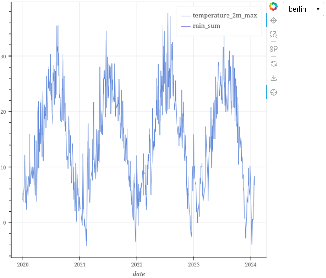
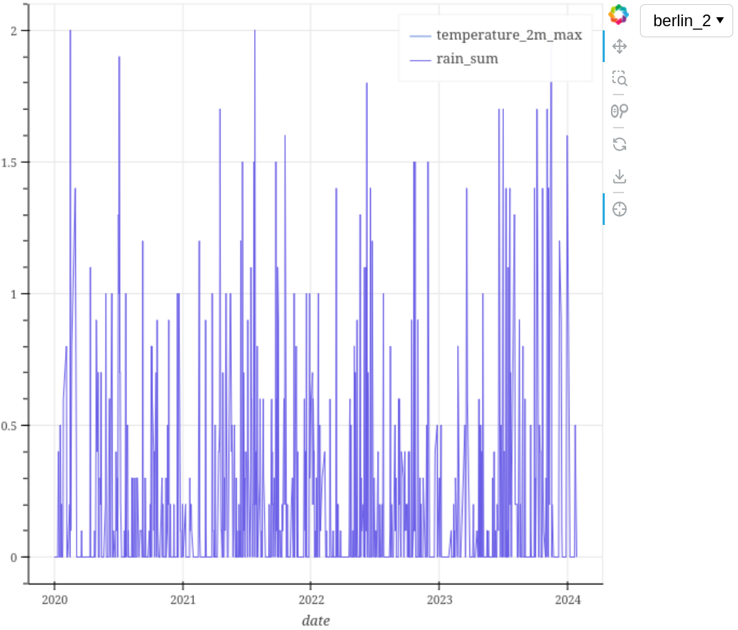
plotting_tool.plot_interactive({
df_name_berlin: ['date', 'temperature_2m_max'],
df_name_berlin_2: ['date', 'rain_sum']})
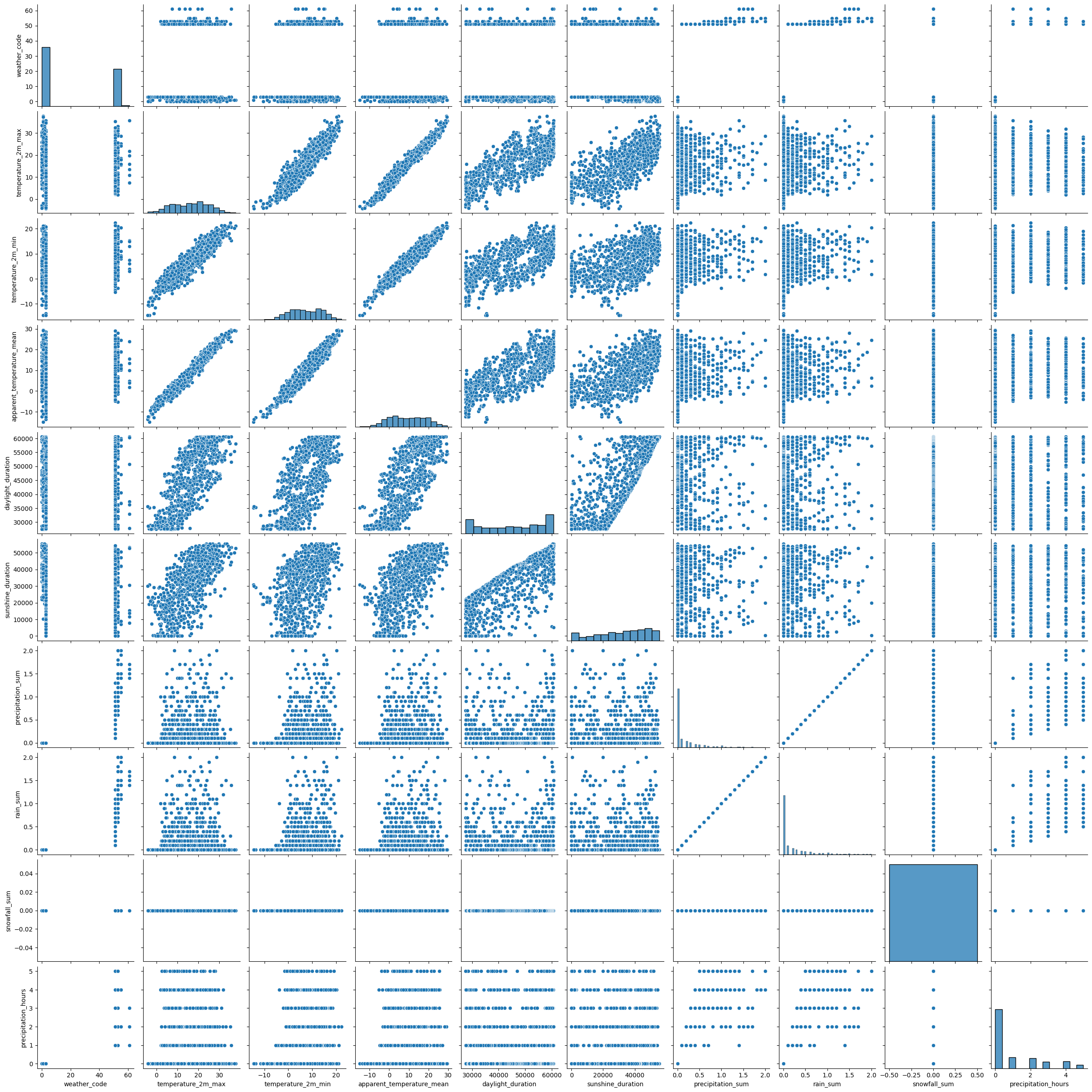
plotting_tool.plot_univariate_graphs(df_name_berlin, number_columns_unvariate_graphs=3)
# In this example the columns used for plotting bivariate graphs
# are the same as the ones to keep
plotting_tool.plot_bivariate_graphs(df_name_berlin, numeric_variables=columns_to_check)
plotting_tool.plot_correlation_heatmap(df_name_berlin, numeric_variables=columns_to_check)
# Create a regression model
target_variable = 'precipitation_sum'
predictor_variables = ['temperature_2m_max',
'temperature_2m_min',
'daylight_duration']
regression_model_summary = plotting_tool.get_regression_model_summary(df_name_berlin, target_variable, predictor_variables, disable_feedback=True)
print(regression_model_summary)


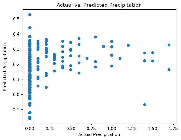
                            OLS Regression Results
==============================================================================
Dep. Variable:      precipitation_sum   R-squared:                       0.098
Model:                            OLS   Adj. R-squared:                  0.094
Method:                 Least Squares   F-statistic:                     27.69
Date:                Wed, 27 Mar 2024   Prob (F-statistic):           5.21e-17
Time:                        12:08:04   Log-Likelihood:                -263.90
No. Observations:                 770   AIC:                             535.8
Df Residuals:                     766   BIC:                             554.4
Df Model:                           3
Covariance Type:            nonrobust
======================================================================================
                         coef    std err          t      P>|t|      [0.025      0.975]
--------------------------------------------------------------------------------------
const                  0.2464      0.059      4.189      0.000       0.131       0.362
temperature_2m_max    -0.0347      0.005     -7.488      0.000      -0.044      -0.026
temperature_2m_min     0.0438      0.005      9.059      0.000       0.034       0.053
daylight_duration   4.189e-06   1.88e-06      2.232      0.026    5.05e-07    7.87e-06
==============================================================================
Omnibus:                      393.491   Durbin-Watson:                   1.990
Prob(Omnibus):                  0.000   Jarque-Bera (JB):             2061.167
Skew:                           2.369   Prob(JB):                         0.00
Kurtosis:                       9.465   Cond. No.                     2.22e+05
==============================================================================

Notes:
[1] Standard Errors assume that the covariance matrix of the errors is correctly specified.
[2] The condition number is large, 2.22e+05. This might indicate that there are
strong multicollinearity or other numerical problems.
Bokeh opens in browser#